Measuring Color Part 1: Setting Up the Problem

This is the story about how a combination of a simple color experiment and limited resources prompted me to design a new experiment and analysis for the lab where I worked. What started as a simple fuel test turned into a project that taught me a great deal about how humans perceive light and color.

The Problem

Suppose you work in a laboratory, and your clients want you to to grade the color of some fuel specimens. They specify that you are supposed to assign a number to the fuel from 1 to 8 ranging from a pale yellow (1), red (4) or nearly black (8), and various shades and numbers in between. Well, it’s good to have clients, and the test sounds simple enough. Great!

But we can’t just eyeball that measurement, and the standard method calls for equipment you don’t have. The lab has limited resources, and you can’t seem to talk your boss into buying the parts you need or turning the clients down. So what do you do?

Opportunity

The standard methods of getting a color measurement require either visual matching to a reference material using a standard light source or use of a specialized piece of equipment. However, visual matching does not leave a quantitative record of the measurement, and we lacked the resources to acquire a specialized instrument. Furthermore, it would be advantageous to analyze colors that fell outside the narrowly-defined yellow-red-black range.

Maybe there was a way to get a measurement that was not only documentable, calibratable, and reproducible, but arguably better than the standard method of visually comparing the specimen to a piece of reference glass!

I found two key resources that would help me escape my conundrum:

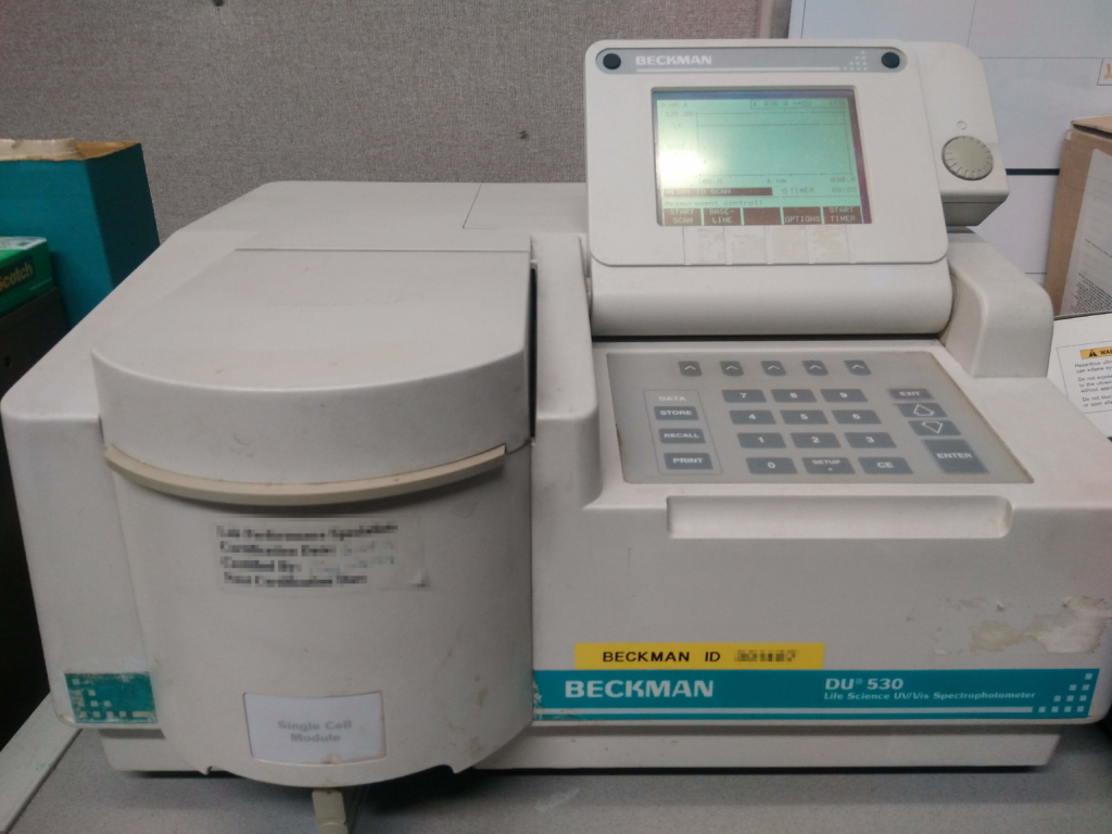
  • The lab had an old, out-of-commission UV/Vis spectrophotometer.
  • ASTM D1500 provides the RGB color values for the different color numbers of specimens observed using a standard light source.
Maybe this old spectrophotometer could find a second life measuring fuel color!

So maybe I could get that spectrophotometer working, convert its output to RGB color values, and match it to the nearest standard color number! Then I would have a quantitative record and the capability to identify colors outside of the standard’s yellow-red-black palette.

The Challenge

So I had a path towards a method that I could feel good putting in front of a client.

  1. Bring the defunct UV/Vis back to life.
  2. Find a way to transfer the UV/Vis spectra to a computer.
  3. Convert a continuous spectrum to RGB space.
  4. Match the RGB coordinates to their nearest standardized color value.

Step 3 is where I will focus this series of blog posts because working on the spectrum → RGB conversion taught me a great deal about human vision and color perception. After all, how does the human eye really perceive the visible spectrum? How is it that we take just red, green, and blue light and still create what appears to be the entire spectrum of visible electromagnetic radiation? How can we convert a continuous spectrum to those 3 color channels?

The next post will get to the heart of the problem: How the continuous visible spectrum relates to the red, green, and blue color channels that humans use in our cameras and displays.

Rules of Exponents

Definitions

Terminology
We would call this “x raised to the a power”
Rules_of_exponents_1.png
x is called the base
a is called the exponent

Example:
Rules_of_exponents_2.png is called “seven raised to the eleventh power”
the base is 7
the exponent is 11

Integer exponents
An integer exponent just means multiplying a number by itself.
Rules_of_exponents_3.png

Example:
Rules_of_exponents_4.png
Rules_of_exponents_5.png

Fraction exponents
An exponent which is the reciprocal of an integer means taking the root
Rules_of_exponents_6.png

Example:
Rules_of_exponents_7.png
Rules_of_exponents_8.png

Negative exponents
A negative exponent indicates a reciprocal
Rules_of_exponents_9.png

Example:
Rules_of_exponents_10.png
Rules_of_exponents_11.png

NOTICE: This means you don’t ever have to deal with fractions or roots ever again if you don’t want to! You can treat them all like exponents.

Algebra rules

Combining exponents
When two numbers with the same base are multiplied, the exponents may be added
Rules_of_exponents_12.png

Example:
Rules_of_exponents_13.png
Rules_of_exponents_14.png

Exponents in ratios
When exponents in the numerator an denominator have the same base, their exponents may be subracted
Rules_of_exponents_15.png

NOTE: This is just a combination of the negative exponent rule with the multiplication rule!

Distributing exponents
If you have 2 layers of exponents, they may be combined
Rules_of_exponents_16.png

Example:
Rules_of_exponents_17.png
Rules_of_exponents_18.png

Negative bases
When the base is a negative number, the sign of the expression overall depends on whether the exponent is even or odd.
Rules_of_exponents_19.png   if n is an odd integer
Rules_of_exponents_20.png   if n is an even integer

Therefore:
Rules_of_exponents_21.png   if n is an odd integer
Rules_of_exponents_22.png   if n is an even integer

Examples:
Rules_of_exponents_23.png
Rules_of_exponents_24.png

A warning about addition
Exponents DO NOT distribute cleanly over addition
Rules_of_exponents_25.png

You either have to find a way to simplify the base first OR use the definition of the exponent to simplify things.
Examples:
Rules_of_exponents_26.png

Rules_of_exponents_27.png

Rules_of_exponents_28.png
Rules_of_exponents_29.png

Algebra: Shifting and scaling functions

Functions of a certain form can be scaled and translated by modifying the constants contained in the expression. Suppose we have some function of x that has not been shifted or scaled in any way.

$$ y = f(x) $$

We can modify that function to be shifted by (h, k) and scaled by the factor a.

$$y = a*f(x-h)+k$$

  • Scaling occurs by simply multiplying the expression by some scale factor. In my examples here, that scale factor is a.
  • Translation left and right can be accomplished by replacing x with (x-h), where h is how far the function is shifted to the right.
  • Translation up and down is accomplished by simply adding a constant k, where k is how far the function is shifted up.

Here is an interactive example showing how a parabolic function may be shifted and scaled. (If the embedded applet isn’t working, you can access it here.)

And here is the scaling of an exponential function.
(If the embedded applet isn’t working, you can access it here.)

You can also play with examples of function shifting and scaling with the Desmos online graphing calculator.

A map of unit conversions and chemical reactions

Recently, a student of mine showed me a way of visualizing and planning out unit conversion-type chemistry problems that I had never seen before, so I made my own version of this visual aid. It is essentially a flow chart illustrating how many stoichiometry and dimensional analysis problems can be mapped out visually as a series of unit conversions.


You can also download a pdf version here.

This tool can be used to visualize a sequence of unit conversions to solve a variety of chemistry problems. Each box represents a quantity, and each arrow shows the conversion factor needed to move from one quantity to the next. Just be sure to use dimensional analysis to make sure the units work out!

Now students can’ t always have this chart on hand, and they will eventually want to move on from this learning aid. So there is an axiom that I think distills the essence of the chart into a single sentence.

When in doubt, convert to moles.

The concept of the mole is central to this entire unit conversion process, so if a student remembers that they can convert to and from moles from mass, volume, and/or the number of particles, then they should be able to solve most problems.

Here are some example stoichiometry problems. Go see if the unit conversion map helps you plan your dimensional analysis-based solution!

There is no comparison between that which is lost by not succeeding and that which is lost by not trying.

Francis Bacon

Forms of Quadratics

You can represent a quadratic equation in a whole lot of different forms. Each has its advantages.

Standard forms let you learn valuable information about an equation just by looking at what number was put where. There are three common forms of quadratic equations, also known as second-order polynomials.

Note that variables like a, b, and c in these descriptions will change in meaning from form to form.

Standard form

$$y=\text{ax}^2+\text{bx}+c$$

Advantage: Relative mathematical simplicity, sets you up to use the quadratic formula, and easy to find the y-intercept. It is just the constant y=c.

Example: $$y=2 x^2+12 x-14$$

Factored form

$$y=a(x+b)(x+c)$$

Advantage: Easy to find the x-intercepts. They are at x=-b and x=-c. You don’t even need the quadratic formula!

Example $$y = 2(x+7)(x-1)$$

Vertex form

$$y=a(x-h)^2+k$$

Advantage: Easy to find the vertex, which is at (h,k).

Example: $$y=2 (x+3)^2-32$$

All three of the examples from this post were actually the same quadratic equation! See if you can identify the vertex, x-intercepts, and y-intercepts using the different forms.

K: The Stress Intensity Factor

Fracture Mechanics is the study of how cracks grow and materials break apart. One of the most important concepts in the world of fracture mechanics is K, the linear-elastic stress intensity factor.

It is easy to confuse what K is used for with what it actually means. K is useful for measuring a material’s resistance to fracture starting at a sharp-tipped crack. However, K is defined as a measurement of the magnitude of stress distribution around a sharp crack tip in a linear-elastic solid. K only has meaning in the context of materials that can be expected to form a certain distribution of stress around a sharp crack tip!

So if we have something that is predominantly linear-elastic (high-strength steels, glass, etc.) and it contains a sharp-tipped crack, then the stress distribution around that crack can be given in terms of this parameter we call K. The stress distributions for a crack in tension perpendicular to the crack faces (aka Mode I loading) are:

$$\sigma _{\text{yy}}=\frac{K
}{\sqrt{2 \pi r}} \cos (\theta ) \left(\sin \left(\frac{\theta }{2}\right) \sin \left(\frac{3 \theta }{2}\right)+1\right)$$

$$\sigma _{\text{xx}}=\frac{K
}{\sqrt{2 \pi r}}
\cos (\theta ) \left(1-\sin \left(\frac{\theta }{2}\right) \sin \left(\frac{3 \theta }{2}\right)\right) $$

$$\sigma _{\text{xy}}=\frac{K
}{\sqrt{2 \pi r}} \left(\sin \left(\frac{\theta }{2}\right) \cos \left(\frac{\theta }{2}\right) \cos \left(\frac{3 \theta }{2}\right)\right)$$

These plots show how the stress distribution looks for a stress intensity factor of K = 1 MPa √m.


Stress distribution for a stress intensity factor of K = 1 MPa √m. The crack tip is located at (0,0) and the crack follows the x-axis along x < 0.

Stress distribution for a stress intensity factor of K = 2 MPa √m. Note that I kept the same scale so that we can see the effect on the spatial distribution.

Hopefully, this helps illustrate what the stress intensity factor, K, means in a mathematical sense. Though K is useful for measuring fracture toughness, it is only applicable for sharp crack tips in linear-elastic materials that exhibit stress distributions similar to what I have shown here.

Note that these solutions are approximations: they are the first, most significant term of a summation. But K is still a very useful parameter for materials that obey linear-elastic fracture mechanics.

I created a live-view applet for Wolfram Cloud, but it wasn’t playing nice with the cloud, hence my screenshots above. In the event I get it working, I’ll put it here.

Ce qui est simple est toujours faux. Ce qui ne l’est pas est inutilisable.
What is simple is always wrong. What is not is unusable.

Paul Valéry

Silly Math Question: Is It Possible to Write Pi Backwards?

This was inspired by the Quora question “What is Pi backwards?” It seemed like a good early post to try converting Mathematica code and LaTeX to WordPress.

The concise answer to the question is “That question is meaningless,” but why is this the case? After all we can write 123 “backwards” as 321, why not π?

One explanation is that π is an irrational number with unlimited digits, and something without an end cannot be reversed. Or something with no end, written backwards, becomes a thing with no beginning. Or one could say that “reversing” any number really doesn’t have much meaning in the first place. Yet, this question gives us a good opportunity to explore what we mean when we describe π as an irrational number.

One way to look at π is as a summation, like this summation equivalent to the arctangent function. $$4*ArcTan(1) = \pi$$

$$4 \sum _{n=1}^{\infty } \frac{(-1)^{n-1}}{2 n-1}=4 \left(1 \frac{1}{1}-\frac{1}{3}+\frac{1}{5}-\frac{1}{7}+\frac{1}{9}\text{…}\right)=\pi$$

If you look at that sum, it adds up an infinite terms, and every term is smaller than the previous one. Thus, every term we evaluate brings us closer to the actual value of π. But, we never run out of terms, so we never find the exact value of π. We just get closer and closer forever.

We can approximate π by going out to 100 terms.

$$4 \sum _{n=1}^{100} \frac{(-1)^{n-1}}{2 n-1} = 3.13159$$

This gets us in the neighborhood. (Note that I rounded to 7 digits.) But we can get closer by going to 1000 terms.

$$4 \sum _{n=1}^{1000} \frac{(-1)^{n-1}}{2 n-1} = 3.14059$$

Now π is starting to look like the number we recognize! If I kept adding more terms, then I would need to round to a larger number of digits to see the change. If we could go forever, the summation converges to π itself. Now you probably have some idea of why approximating π to a certain number of digits is such a popular problem to throw at big computers.

This sets us up to see why “π backwards” ends up being meaningless. The number has no end, so there is nowhere to “start” the reverse-order number. Just for fun, though, we can interpret “π backwards” as an excuse to switch the starting and ending place of the summation.

$$4 \sum _{n=\infty }^1 \frac{(-1)^{n-1}}{2 n-1}=\pm 4\left(\frac{1}{2 \infty -1}-\frac{1}{2 \infty -3}+\frac{1}{2 \infty -5}\text{…}\right)$$

Notice that we are starting at infinity, so we will never reach a definite answer to this summation either. But it’s worse than that. We are effectively dividing by infinity in every term, so every term is practically zero. We can’t even figure out if the “first” term is positive or negative! (Not that it really matters when every term is zero.)

$$4 \sum _{n=\infty }^1 \frac{(-1)^{n-1}}{2 n-1}= \pm 4\left(\frac{1}{\infty }-\frac{1}{\infty }+\frac{1}{\infty }\right) =\pm (0-0+0\text{…})$$

So we do have an answer for what “Pi backwards” might look like. Every term is effectively zero, yet infinitesimally larger than the previous term, we can’t even figure out the sign of the terms, and there is an infinite number of these infinitely insignificant terms to add up. We will never get to a term that isn’t zero because by starting at the “infinity” term, we put ourselves infinitely far away the “end” of our summation.

So “Pi backwards” looks like an infinite summation of zeroes. At least looking at π forwards gave us a reasonable approximation of the actual number because it prioritized the largest, most significant terms.

Film is one of the three universal languages, the other two: mathematics and music.

Frank Capra

A Blog is Born!

Welcome to my new website! I am Wade Lanning, a materials scientist, lab manager, and teacher. This will be my platform for sharing my various projects and lessons, and hopefully, this post is the first of many!

So get ready for a stream of whatever I happen to be doing any given week! Right now, I am working primarily as a tutor, and most of my posts will be based on lessons I prepared for my students. However, you can also expect snippets of my past research, miscellaneous mini-projects, photos, or whatever I happen to be working on that day.

Progress lies not in enhancing what is, but in advancing toward what will be.

Khalil Gibran